Distribution of height & weight in sumo divisions

library(tidyverse)
## Warning: package 'tidyr' was built under R version 4.0.3

Now that we’ve downloaded sumo data let’s have a look at sumo wrestlers’ height and weight.

Read banzuke.csv with hard-coded column types:

df <- read_csv(
    "banzuke.csv",
    col_types = "ciccccDddcii"
)

The dataset goes a long way back:

df %>% 
    summarise_at(
        vars(basho),
        c("min", "max")
    )
## # A tibble: 1 x 2
##   min     max    
##   <chr>   <chr>  
## 1 1983.01 2020.11

First one or two letters in the rank column indicate which of sumo divisions the wrestler belongs to:

divisions <- c("Jk", "Jd", "Sd", "Ms", "J", "M", "K", "S", "O", "Y")

df %>% 
    mutate(
        division = str_extract(
            rank,
            "^\\D+")
    ) %>% 
    mutate_at(
        vars(division),
        ordered,
        levels = divisions
    ) %>% 
    count(division)
## # A tibble: 10 x 2
##    division     n
##    <ord>    <int>
##  1 Jk       18727
##  2 Jd       60908
##  3 Sd       45090
##  4 Ms       27193
##  5 J         6072
##  6 M         6853
##  7 K          478
##  8 S          495
##  9 O          810
## 10 Y          489

To keep things simple, let’s put komusubi, sekiwake, ōzeki and yokozuna in “M” division:

df <- df %>% 
    mutate(
        division = str_extract(
            rank,
            "^\\D+"
        )
    ) %>% 
    mutate_at(
        vars(division),
        recode,
        K = "M", S = "M", O = "M", Y = "M"
    ) %>% 
    mutate_at(
        vars(division),
        ordered,
        levels = head(divisions, -4)
    )

df %>% 
    count(division)
## # A tibble: 6 x 2
##   division     n
##   <ord>    <int>
## 1 Jk       18727
## 2 Jd       60908
## 3 Sd       45090
## 4 Ms       27193
## 5 J         6072
## 6 M         9125

There are a few records with missing height/weight in lower divisions, but that’s unlikely to introduce any bias:

df %>% 
    group_by(division) %>% 
    summarise(
        total = n(),
        no_height = sum(is.na(height)),
        no_weight = sum(is.na(weight)),
        .groups = "drop"
    )
## # A tibble: 6 x 4
##   division total no_height no_weight
##   <ord>    <int>     <int>     <int>
## 1 Jk       18727      2843      2843
## 2 Jd       60908      2132      2132
## 3 Sd       45090       123       123
## 4 Ms       27193        74        74
## 5 J         6072         2         2
## 6 M         9125         0         0

Now, this is interesting – higher the division, taller the average wrestler:

df %>% 
    drop_na(height) %>% 
    ggplot(
        aes(
            height,
            colour = division
        )
    ) +
        geom_density() +
        scale_colour_brewer(
            palette = "Greys"
        ) +
        theme_minimal()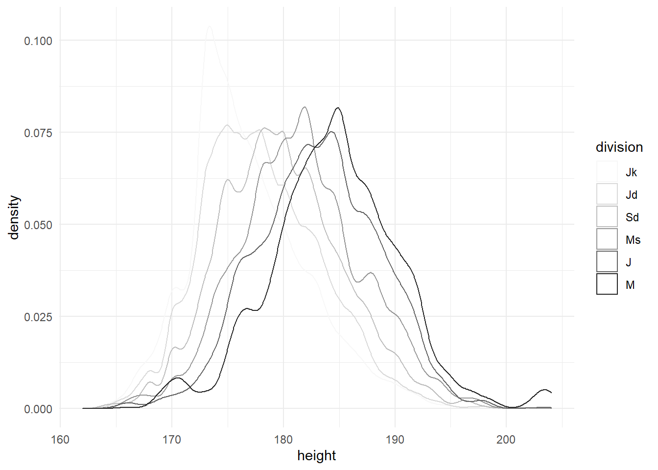

Increase in average weight is less of a surprise:

df %>% 
    drop_na(weight) %>% 
    ggplot(
        aes(
            weight,
            colour = division
        )
    ) +
        geom_density() +
        scale_colour_brewer(palette = "Greys") +
        theme_minimal()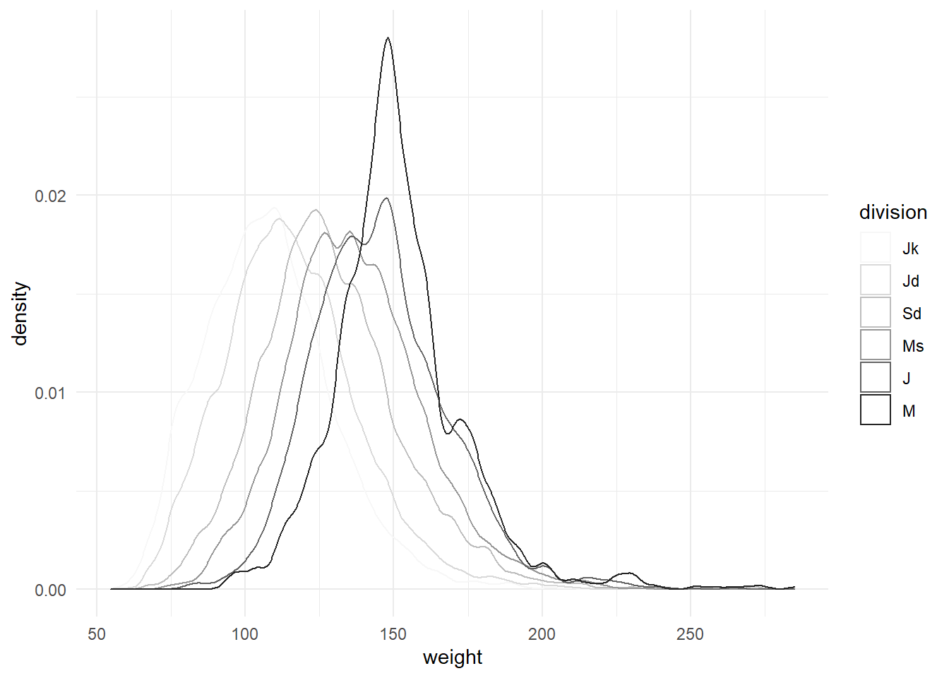

Calculating mean or median (to reduce the influence of outliers) yields neatly increasing figures:

df %>% 
    group_by(division) %>% 
    summarise_at(
        vars(
            height,
            weight
        ),
        median,
        na.rm = TRUE
    )
## # A tibble: 6 x 3
##   division height weight
##   <ord>     <dbl>  <dbl>
## 1 Jk         176    106.
## 2 Jd         178.   114 
## 3 Sd         180.   126.
## 4 Ms         182.   135.
## 5 J          183    144 
## 6 M          185    149